A typical application of deep learning is image classification. The use of deep learning techniques for image classification has performed well, even exceeding the human level. However, there is no free lunch in the world. Deep learning also imposes severe demands on the resources of computational resources. However, in some resource-constrained scenarios, it is still necessary to apply deep learning for image classification. This is a huge technical challenge.
Resource-constrained scenario
There are a number of resource-constrained scenarios, the most important of which are:
The performance limit of the device itself, such as mobile devices.
Massive Data. Many large companies have massive images that need to be processed, and there is an urgent need to optimize performance while maintaining classification accuracy.
The former commonly used setting is anytime classification. For example, using a mobile phone to shoot a flower, the deep learning model may return a rough classification result of "flower" first, and recognize that this is taking flowers and calling the corresponding scene patterns (for example, macro flowers). If the user stays in the current interface for a long time after shooting, the model further returns the specific type of flower (the user may want to know what flower was just taken). If you go directly back to a specific category, it may take a long time. At this time, the user may have already pressed the shutter, too late to call the corresponding scene mode.
In addition to the above scenarios, another typical application scenario of anytime classification is to adapt different devices. There are a variety of mobile devices with different capabilities. Anytime classification means that we only need to train one model and then deploy it to different devices. On poorly performing devices, the model gives a rough classification. On a device with better performance, the model gives a fine classification. In this way, we do not need to train models for all kinds of strange models.
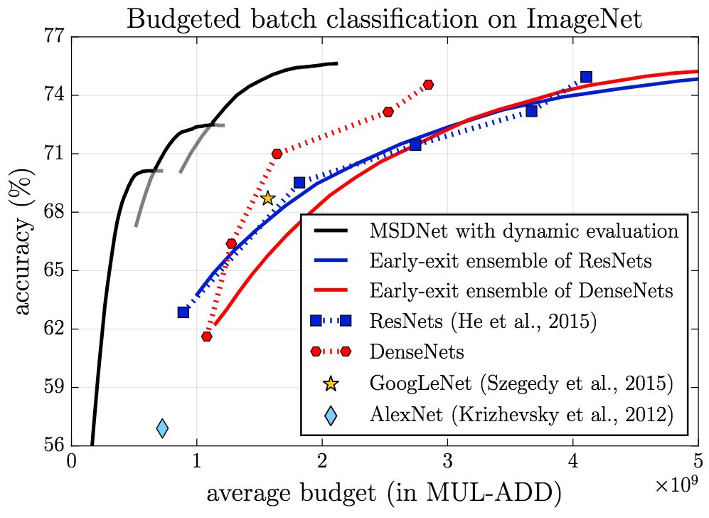
The latter common setting is budgeted batch classification. Unlike anytime classification, this time limit is not on a single image (for example, before the user presses the shutter), but on the entire batch of images. For this scene, the classification of the images to be processed is not necessarily the same.
For example, the horse on the left side of the figure is well-detected, and even a simple network can detect it. The right horse, because of the shooting angle relationship, is not easy to detect and requires a heavy burden on the network architecture.
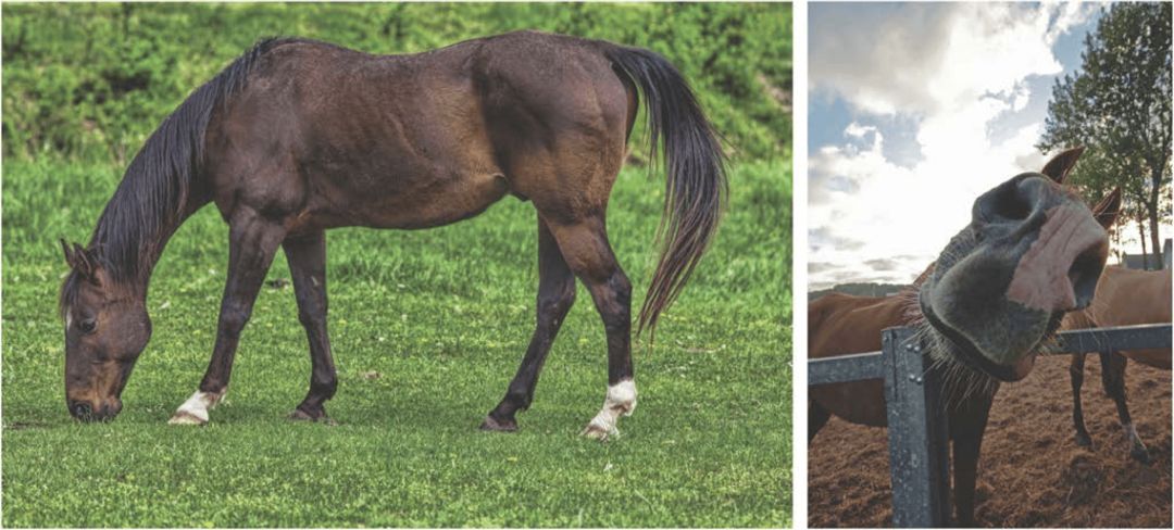
Image Credit: Pixel Addict and Doyle; License: CC BY-ND 2.0
If the entire batch of images is classified using simple models, some images cannot be classified correctly. On the contrary, if the entire batch of images are classified using complex models, then a lot of resources are wasted on simple images. Therefore, we need a flexible model that can use either fewer resources for rough classification or more resources for fine classification.
We have seen that both the anytime classification and the budgeted batch classification require the model to have both rough classification and fine classification. So, although the two scenes on the surface are very different (a typical application scenario is single image classification on mobile devices, and another typical application scenario is mass image classification on large companies' high-performance devices), its internal The consistency of requirements means that we can build a unified model to meet the challenges of these two scenarios (or, at the very least, the general idea of ​​a consistent model architecture, and then make local adjustments based on the differences between these two scenarios).
Model intuition
The simplest and straightforward solution to the above-mentioned problem is to use multiple different networks, each with different capabilities (the corresponding computational needs are also different). Specifically, using a group of networks, the capabilities of each network are sequentially increased. Then use this group of networks in order to sort. In the anytime classification scenario, the latest classification result is returned. In the case of budgeted batch classification, when the confidence level of the results of the network is high enough, the result is returned, and then the subsequent network is skipped and the next image is directly classified.
This program is very straightforward, easy to understand and easy to implement. The problem is that many of the work done by multiple models is repetitive (for example, features that need to be extracted through convolutional layers), and multiple models cannot be reused, and each model must be started from scratch. For a resource-constrained environment, such waste is unacceptable.
In order to achieve multiplexing, multiple networks can be integrated into one model and share many components, resulting in a deep network based on cascading classification layers.
However, the CNN (convolutional neural network) architecture was originally not designed for this cascade, so such a simple stacking classification layer leads to two problems:
Different layers of the CNN extract image features at different scales. In general, the front layer extracts the fine features (local), while the back layer extracts the rough features (the whole). The classification is highly dependent on the overall rough features. The previous classification layer was very poor because of the lack of features on the coarse scale.
The added classification layer may interfere with the feature extraction layer. In other words, the front classification layer may affect the effectiveness of the final classification layer.
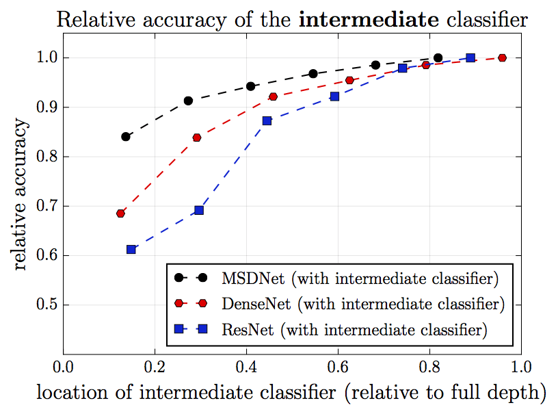
The following figure shows the comparison of the classification results of different network architectures on the CIFAR-100. Among them, the vertical axis is relative accuracy (accuracy of the final classification layer is 1), and the horizontal axis is the relative position of the intermediate classification layer (the position of the final classification layer is 1). Black represents MSDNet (new proposed architecture), red represents DenseNet, and blue represents ResNet (as a comparison object). We see that the more backward the classification layer, the higher the accuracy of the classification. However, in DenseNet and ResNet, the top few classification layers perform particularly poorly, and there is a big gap with the latter. This is particularly evident on ResNet. This is precisely because the top few classification layers lack features on a coarse scale.
Look at a picture again. In this figure, each time an intermediate classification layer is inserted in the network, the horizontal axis represents the position of the inserted single intermediate classification layer, and the vertical axis represents the performance of the corresponding final classification layer. We see that in ResNet, the more advanced the middle layer is inserted, the worse the performance of the final classification layer will be. This is because the inserted classification layer interferes with the operation of the feature extraction layer. The more advanced the insertion is, the worse the performance of the final classification layer is. This is probably because the more the classification layer is inserted, the closer the corresponding feature extraction layer is to the performance of the closer intermediate classification layer. The “short-term goals†are optimized, and correspondingly the need for the “long-term goal†of the longer final classification layer is ignored.

So how do you deal with these two issues?
We first consider the second problem, the classification layer interference problem. As mentioned earlier, the feature extraction layer is optimized for the closer intermediate classification layer, ignoring the need for a further final classification layer. So, if we connect the feature extraction layer with the later classification layer? With the direct connection between the feature extraction layer and the subsequent classification layer, it is not possible to avoid the optimization of the classification layer that is too advanced, and to ignore the later classification layer. In fact, DenseNet published by Gao Huang et al. at CVPR 2017 provides such features.
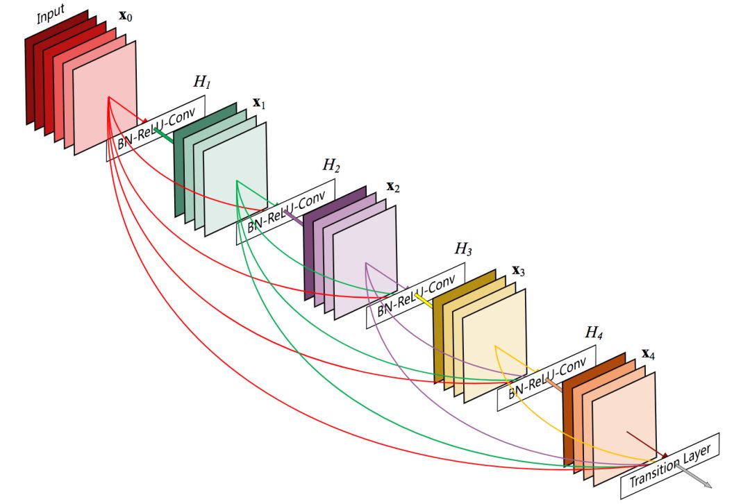
5-layer DenseNet components
The previous picture also shows that, under DenseNet, inserting the classification layer in front of it has little effect on the final classification layer.
As for the first problem that lacks coarse-scale features, it can be solved by maintaining a multi-scale feature map.
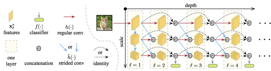
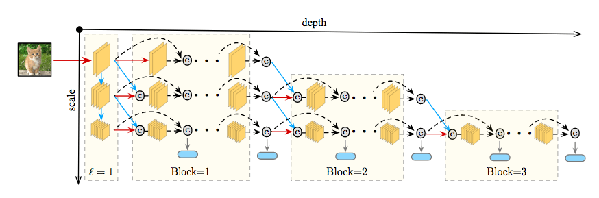
In the figure above, the depth is deeper from left to right, the scale is from top to bottom, from fine to coarse, and all classifiers use the features of the rough layer (the rough layer is related to the classification height). Characteristic maps on specific layers and scales are calculated by connecting one or two of the following convolutions:
The result of the usual convolution operation of the previous layer on the same scale (horizontal red line in the figure)
(If possible,) step convolution operation of feature mapping on a finer scale in the previous layer (blue line diagonally in the figure).
Combining these two types, the Multi-Scale Dense Network (abbreviated as MSDNet) is obtained.
MSDNet architecture
As shown earlier, the architecture of MSDNet is as follows:

The first layer The first layer (l=1) is special because it contains vertical connections (blue lines in the figure). Its main role is to provide representation "seeds" on all scales. The coarse-scale feature map is obtained by downsampling.
Subsequent Layers Subsequent layers follow the structure of DenseNet, and the connection of feature maps at specific layers and scales is described in the previous section. The output of the first and subsequent layers is detailed in the figure below.
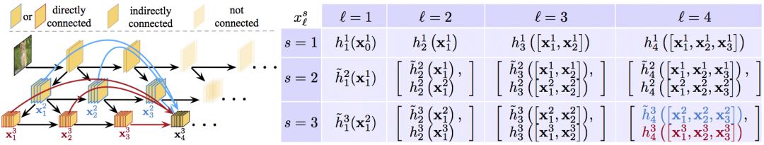
The classifier classifier also follows DenseNet's dense connection model. Each classifier consists of two convolution layers, an average pooling layer, and a linear layer. As described above, in the anytime setting, the latest forecast is output when the budget time is exhausted. Under the batch budget setting, the classifier fk exits when its prediction confidence (the maximum value of the softmax probability) exceeds a predefined threshold θk. Prior to training, the computational cost Ck of the network reaching the k-th classifier is calculated. Correspondingly, the probability that a sample exits at the classifier k is qk = z(1-q)k-1q. where q is the exit probability that the sample arrives at the classifier and a class with sufficient confidence is obtained and exited. We assume that q is constant on all layers. z is a normalization constant that ensures that ∑kp(qk) = 1. When testing, it is necessary to ensure that the total overhead of all samples in the classification test set Dtest does not exceed the expected budget B. This is the limit of |Dtest|∑kqkCk ≤ B. We can solve the q-value of this constraint on the verification set, and then decide θk.
Loss function In training, all classifiers use the cross-entropy loss function L(fk) and minimize the weighted cumulative loss:
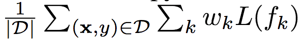
In the above formula, D is the training set, wk is the weight of the k-th classifier, and wk ≥ 0. If the budget distribution P(B) is known, we can use the weight wk to combine the prior knowledge about budget B. In practice, we have found that all loss functions use the same weighting effect.
Network Simplification and Inert Calculations The above network architecture can be further simplified by two straightforward methods. First, maintaining all dimensions at each level is not efficient. A simple strategy to reduce the network size is to divide the network into S blocks, leaving only the coarsest (S - i + 1) scale in the i-th block. While removing the scale, a corresponding transition layer is added between the blocks, 1x1 convolution is used to merge the connected features, and half of the channels are intercepted before passing the fine-scale features to the coarse scale through step convolution.
Second, because the layer 1 classifier uses only the features of the coarsest scale, the finer feature map of the layer 1 (and some of the finer feature maps before the S-2 layer) does not affect the classifier's prediction. Therefore, propagating the sample along the path required by the next classifier can minimize unnecessary calculations. The researchers call this strategy lazy calculus.
test
data set
The researchers evaluated the effect of MSDNet on three image classification data sets:
CIFAR-10
CIFAR-100
ILSVRC 2012 (ImageNet)
The CIFAR data set includes 50,000 training images and 10,000 test images with an image size of 32x32 pixels. The researchers left 5,000 training images as verification sets. CIFAR-10 contains 10 classifications and CIFAR-100 contains 100 classifications. The researchers applied standard data enhancement techniques: the image was zeroed on each side with 4 pixels, and then randomly cut to get a 32x32 image. The image is flipped at a 0.5 probability level and normalized by subtracting the channel mean and dividing by the channel's standard deviation.
The ImageNet dataset contains 1000 categories, totaling 1.2 million training images and 50,000 verification images. The researchers retained 50,000 training images to estimate the MSDNet's classifier confidence threshold. The researchers applied the data enhancement techniques proposed by Kaiming He et al. in Deep Residual Learning for Image Recognition (arXiv: 1512.003385). During the test, the image was scaled to 256x256 pixels and then centrally cut to 224x224 pixels.
Training details on the CIFAR dataset, all models (including baseline models) use stochastic gradient descent (SGD) training, mini-batch size is 64. Nestorov momentum method is used, momentum weight is 0.9 (without suppression), weight attenuation is 10-4. All models trained 300 epochs with an initial learning rate of 0.1, divided by 150 after epochs of 150 and 225. ImageNet's optimization plan was similar except that the mini-batch size increased to 256, and all models trained 90 epochs at 30. After 60 epochs and lower learning rate.
The MSDNet for the CIFAR dataset uses 3 dimensions. The first layer uses a 3x3 convolutional (Conv), group normalization (BN), and ReLU activation. Subsequent layers follow DenseNet's design and Conv(1x1)-BN-ReLU-Conv(3x3)-BN-ReLU. The output channels on the three scales are 6, 12, and 24, respectively. Each classifier contains 2 downsamples. Convolutional layer (128 dimensional 3x3 filter), 1 2x2 averaged pooled layer, 1 linear layer.
MSDNet for ImageNet uses four dimensions, and accordingly, each layer generates 16, 32, 64, 64 feature maps. Before passing into layer 1 of MSDNet, the original image is first transformed through 7x7 convolution and 3x3 maximum pooling (in steps of 2). The structure of the classifier is the same as for MSDNet for CIFAR, except that the number of output channels per convolutional layer is the same as the number of input channels.
On the CIFAR data set, MSDNet for anytime setting has 24 layers. The classifier operates on the output of the 2x(i+1) layer, where i=1,..., 11. The MSDNet depth for the budgeted batch setting is 10 to 36 layers. The k-th classifier is located in the first (∑ki=1i) layer.
MSDNet (anytime and budgeted batch settings) on ImageNet uses 4 scales. Accordingly, the i-th classifier operates on the output of the (kxi+3) th layer, where i=1,...,5,k=4 ,6,7.
ResNet has 62 layers and each resolution contains 10 residual blocks (3 resolutions in total). The researchers trained intermediate classifiers in the 4th and 8th residual blocks of each resolution for a total of 6 intermediate classifiers (plus the final classifier).
DenseNet has 52 layers and contains 3 dense blocks, each with 16 layers. Six intermediate layers are located on the 6th and 12th layers of each block.
All models are implemented using the Torch framework. See GitHub (gaohuang/MSDNet) for code.
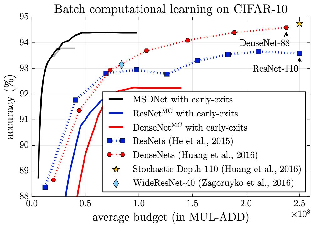
CIFAR-10
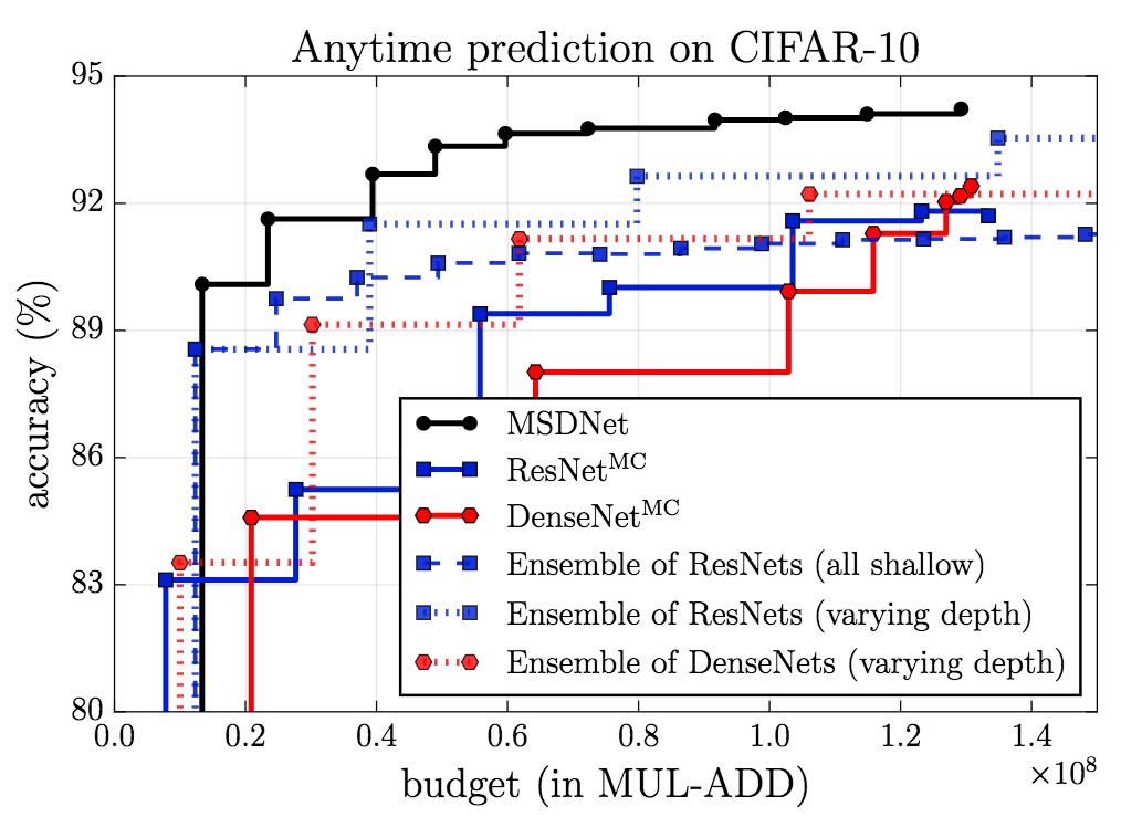
On CIFAR-10, the performance (accuracy) of MSDNet significantly exceeds the baseline both in the setting of anytime and in the budgeted batch setting.
CIFAR-100
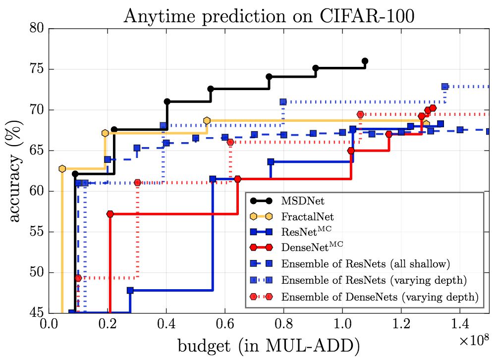
The figure above shows the results of anytime setting. It can be seen that MSDNet performed better than other models except in a very small budget. In the case of a very small budget, the integration method has an advantage because the prediction is made by the first (small) network that is optimized for the very small budget.
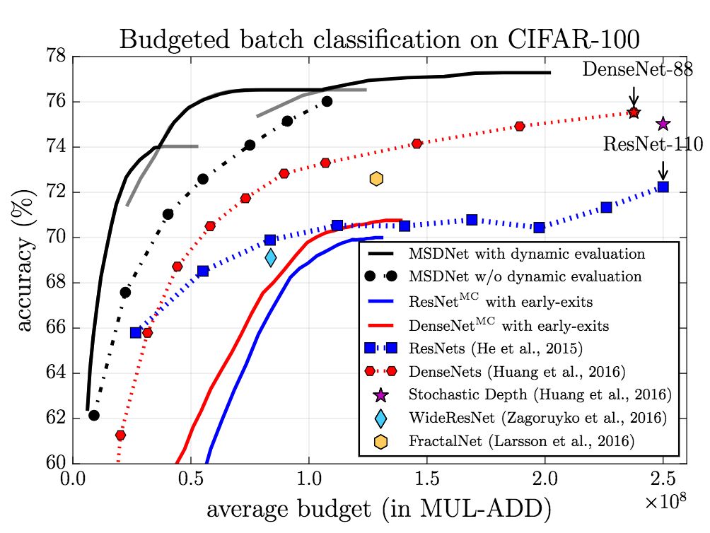
In the budgeted batch setting, MSDNet performed better than other models. Of particular note is that MSDNet uses only one-tenth of the ResNet's 110-bit computing budget to achieve a considerable performance.
ImageNet
MSDNet's performance on ImageNet is equally impressive.
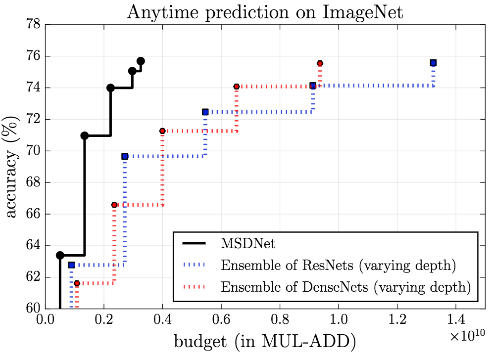
Anytime
Budgeted batch
Ablation test
Ablation tests verify the effectiveness of dense connections, multiscale features, and intermediate classifiers.
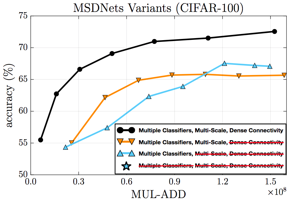
Ablation test on CIFAR-100
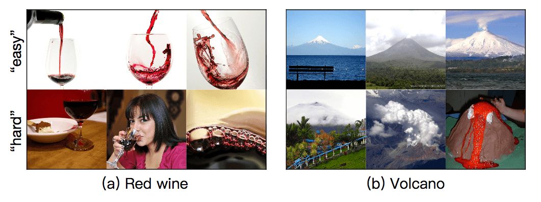
In addition, the researchers randomly selected some images from ImageNet. The figure below is divided into two lines. The image on the top line is easy to classify, and the image on the bottom line is more difficult to classify. MSDNet's first classifier correctly predicted the classification of "easy" images, but failed to predict the classification of "difficult" images. MSDNet's final classifier correctly predicted the classification of "difficult" images.
Conclusion
At the just-concluded ICLR 2018, the author of this article gave an oral report (May 1 04:00 -- 04:15 PM; Exhibition Hall A).
Researchers intend to further explore resource-constrained depth architectures beyond classification, such as image segmentation. In addition, researchers are also interested in exploring more ways to further optimize MSDNet, such as model compression, spatial adaptive computing, and more efficient convolution operations.
Calcium fluoride is often used in spectroscopic windows and lenses due to its high transmission from 200nm to 7μm. Its low absorption and high damage threshold makes it a popular choice for excimer laser optics. Calcium fluoride's low index of refraction allows it to be used without an anti-reflective coating. The Knoop hardness of calcium fluoride is 158.3. Calcium Fluoride (CaF2) Windows manufactured from vacuum UV grade calcium fluoride are commonly found in cryogenically cooled thermal imaging systems.
Caf2 Windows and Lens,Ir Caf2 Windows,Ir Caf2 Lens Single,Crystal Caf2 Windows
Zoolied Inc. , https://www.zoolied.com